Playing with Importance Sampling
Our goal over the next several chapters is to instrument our program to send a bunch of extra rays toward light sources so that our picture is less noisy. Let’s assume we can send a bunch of rays toward the light source using a PDF $\operatorname{pLight}(\omega_o)$. Let’s also assume we have a PDF related to $operatorname{pScatter}$, and let’s call that $operatorname{pSurface}(\omega_o)$. A great thing about PDFs is that you can just use linear mixtures of them to form mixture densities that are also PDFs. For example, the simplest would be:
$$ p(\omega_o) = \frac{1}{2} \operatorname{pSurface}(\omega_o) + \frac{1}{2} \operatorname{pLight}(\omega_o)$$
As long as the weights are positive and add up to one, any such mixture of PDFs is a PDF. Remember, we can use any PDF: all PDFs eventually converge to the correct answer. So, the game is to figure out how to make the PDF larger where the product
$$ \operatorname{pScatter}(\mathbf{x}, \omega_i, \omega_o) \cdot
    \operatorname{Color}_i(\mathbf{x}, \omega_i) $$
is largest. For diffuse surfaces, this is mainly a matter of guessing where $\operatorname{Color}_i(\mathbf{x}, \omega_i)$ is largest. Which is equivalent to guessing where the most light is coming from.
For a mirror, $\operatorname{pScatter}()$ is huge only near one direction, so $\operatorname{pScatter}()$ matters a lot more. In fact, most renderers just make mirrors a special case, and make the $\operatorname{pScatter}()/p()$ implicit -- our code currently does that.
Returning to the Cornell Box
Let’s adjust some parameters for the Cornell box:
At 600×600 my code produces this image in 15min on 1 core of my Macbook:
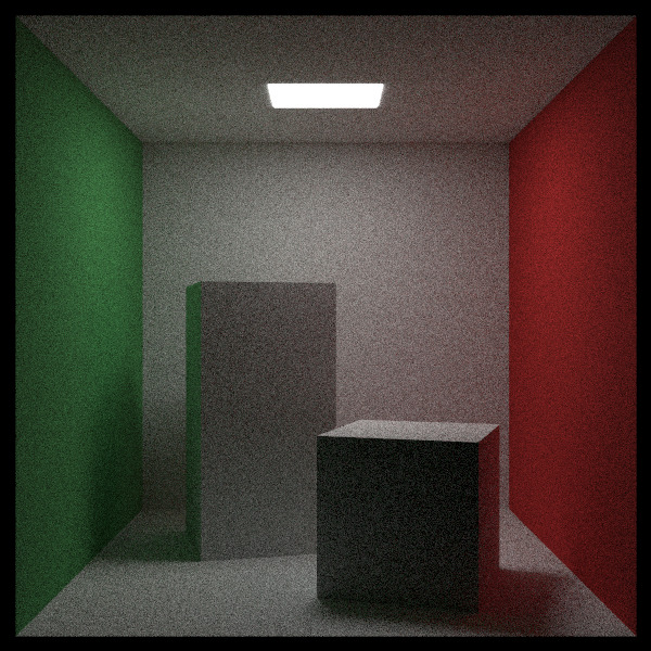
Reducing that noise is our goal. We’ll do that by constructing a PDF that sends more rays to the light.
First, let’s instrument the code so that it explicitly samples some PDF and then normalizes for that. Remember Monte Carlo basics: $\int f(x) \approx \sum f(r)/p(r)$. For the Lambertian material, let’s sample like we do now: $p(\omega_o) = \cos(\theta_o) / \pi$.
We modify the base-class material to enable this importance sampling:
class material {
  public:
    ...

    virtual double scattering_pdf(const ray& r_in, const hit_record& rec, const ray& scattered)
    const {
        return 0;
    }
};
And the lambertian material becomes:
class lambertian : public material {
  public:
    lambertian(const color& a) : albedo(make_shared<solid_color>(a)) {}
    lambertian(shared_ptr<texture> a) : albedo(a) {}

    bool scatter(const ray& r_in, const hit_record& rec, color& attenuation, ray& scattered)
    const override {
        auto scatter_direction = rec.normal + random_unit_vector();

        // Catch degenerate scatter direction
        if (scatter_direction.near_zero())
            scatter_direction = rec.normal;

        scattered = ray(rec.p, scatter_direction, r_in.time());
        attenuation = albedo->value(rec.u, rec.v, rec.p);
        return true;
    }

    double scattering_pdf(const ray& r_in, const hit_record& rec, const ray& scattered) const {
        auto cos_theta = dot(rec.normal, unit_vector(scattered.direction()));
        return cos_theta < 0 ? 0 : cos_theta/pi;
    }

  private:
    shared_ptr<texture> albedo;
};
And the camera::ray_color function gets a minor modification:
class camera {
  ...
  private:
    ...
    color ray_color(const ray& r, int depth, const hittable& world) const {
        hit_record rec;

        // If we've exceeded the ray bounce limit, no more light is gathered.
        if (depth <= 0)
            return color(0,0,0);

        // If the ray hits nothing, return the background color.
        if (!world.hit(r, interval(0.001, infinity), rec))
            return background;

        ray scattered;
        color attenuation;
        color color_from_emission = rec.mat->emitted(rec.u, rec.v, rec.p);

        if (!rec.mat->scatter(r, rec, attenuation, scattered))
            return color_from_emission;

        double scattering_pdf = rec.mat->scattering_pdf(r, rec, scattered);
        double pdf = scattering_pdf;

        color color_from_scatter =
            (attenuation * scattering_pdf * ray_color(scattered, depth-1, world)) / pdf;

        return color_from_emission + color_from_scatter;
    }
};
You should get exactly the same picture. Which should make sense, as the scattered part of
ray_color is getting multiplied by scattering_pdf / pdf, and as pdf is equal to
scattering_pdf is just the same as multiplying by one.
Using a Uniform PDF Instead of a Perfect Match
Now, just for the experience, let's try using a different sampling PDF. We'll continue to have our reflected rays weighted by Lambertian, so $\cos(\theta_o)$, and we'll keep the scattering PDF as is, but we'll use a different PDF in the denominator. We will sample using a uniform PDF about the hemisphere, so we'll set the denominator to $1/2\pi$. This will still converge on the correct answer, as all we've done is change the PDF, but since the PDF is now less of a perfect match for the real distribution, it will take longer to converge. Which, for the same number of samples means a noisier image:
class camera {
  ...
  private:
    ...
    color ray_color(const ray& r, int depth, const hittable& world) const {
        hit_record rec;

        // If we've exceeded the ray bounce limit, no more light is gathered.
        if (depth <= 0)
            return color(0,0,0);

        // If the ray hits nothing, return the background color.
        if (!world.hit(r, interval(0.001, infinity), rec))
            return background;

        ray scattered;
        color attenuation;
        color color_from_emission = rec.mat->emitted(rec.u, rec.v, rec.p);

        if (!rec.mat->scatter(r, rec, attenuation, scattered))
            return color_from_emission;

        double scattering_pdf = rec.mat->scattering_pdf(r, rec, scattered);
        double pdf = 1 / (2*pi);

        color color_from_scatter =
            (attenuation * scattering_pdf * ray_color(scattered, depth-1, world)) / pdf;

        return color_from_emission + color_from_scatter;
    }
You should get a very similar result to before, only with slightly more noise, it may be hard to see.

Make sure to return the PDF to the scattering PDF.
...

double scattering_pdf = rec.mat->scattering_pdf(r, rec, scattered);
double pdf = scattering_pdf;

...
Random Hemispherical Sampling
To confirm our understanding, let's try a different scattering distribution. For this one, we'll attempt to repeat the uniform hemispherical scattering from the first book. There's nothing wrong with this technique, but we are no longer treating our objects as Lambertian. Lambertian is a specific type of diffuse material that requires a $\cos(\theta_o)$ scattering distribution. Uniform hemispherical scattering is a different diffuse material. If we keep the material the same but change the PDF, as we did in last section, we will still converge on the same answer, but our convergence may take more or less samples. However, if we change the material, we will have fundamentally changed the render and the algorithm will converge on a different answer. So when we replace Lambertian diffuse with uniform hemispherical diffuse we should expect the outcome of our render to be materially different. We're going to adjust our scattering direction and scattering PDF:
class lambertian : public material {
  public:
    lambertian(const color& a) : albedo(make_shared<solid_color>(a)) {}
    lambertian(shared_ptr<texture> a) : albedo(a) {}

    bool scatter(const ray& r_in, const hit_record& rec, color& attenuation, ray& scattered)
    const override {
        auto scatter_direction = random_in_hemisphere(rec.normal);

        // Catch degenerate scatter direction
        if (scatter_direction.near_zero())
            scatter_direction = rec.normal;

        scattered = ray(rec.p, scatter_direction, r_in.time());
        attenuation = albedo->value(rec.u, rec.v, rec.p);
        return true;
    }


    double scattering_pdf(const ray& r_in, const hit_record& rec, const ray& scattered) const {
        return 1 / (2*pi);
    }

    ...
This new diffuse material is actually just $p(\omega_o) = \frac{1}{2\pi}$ for the scattering PDF. So our uniform PDF that was an imperfect match for Lambertian diffuse is actually a perfect match for our uniform hemispherical diffuse. When rendering, we should get a slightly different image.
It’s pretty close to our old picture, but there are differences that are not just noise. The front of the tall box is much more uniform in color. If you aren't sure what the best sampling pattern for your material is, it's pretty reasonable to just go ahead and assume a uniform PDF, and while that might converge slowly, it's not going to ruin your render. That said, if you're not sure what the correct sampling pattern for your material is, your choice of PDF is not going to be your biggest concern, as incorrectly choosing your scattering function will ruin your render. At the very least it will produce an incorrect result. You may find yourself with the most difficult kind of bug to find in a Monte Carlo program -- a bug that produces a reasonable looking image! You won’t know if the bug is in the first version of the program, or the second, or both!
Let’s build some infrastructure to address this.