Monte Carlo Integration on the Sphere of Directions
In chapter One Dimensional Monte Carlo Integration we started with uniform random numbers and slowly, over the course of a chapter, built up more and more complicated ways of producing random numbers, before ultimately arriving at the intuition of PDFs, and how to use them to generate random numbers of arbitrary distribution.
All of the concepts covered in that chapter continue to work as we extend beyond a single dimension. Moving forward, we might need to be able to select a point from a two, three, or even higher dimensional space and then weight that selection by an arbitrary PDF. An important case of this--at least for ray tracing--is producing a random direction. In the first two books we generated a random direction by creating a random vector and rejecting it if it fell outside of the unit sphere. We repeated this process until we found a random vector that fell inside the unit sphere. Normalizing this vector produced points that lay exactly on the unit sphere and thereby represent a random direction. This process of generating samples and rejecting them if they are not inside a desired space is called the rejection method, and is found all over the literature. The method covered last chapter is referred to as the inversion method because we invert a PDF.
Every direction in 3D space has an associated point on the unit sphere and can be generated by solving for the vector that travels from the origin to that associated point. You can think of choosing a random direction as choosing a random point in a constrained two dimensional plane: the plane created by mapping the unit sphere to Cartesian coordinates. The same methodology as before applies, but now we might have a PDF defined over two dimensions. Suppose we want to integrate this function over the surface of the unit sphere:
$$ f(\theta, \phi) = cos^2(\theta) $$
Using Monte Carlo integration, we should just be able to sample $\cos^2(\theta) / p(r)$, where the
$p(r)$ is now just $p(direction)$. But what is direction in that context? We could make it based
on polar coordinates, so $p$ would be in terms of $\theta$ and $\phi$ for $p(\theta, \phi)$. It
doesn't matter which coordinate system you choose to use. Although, however you choose to do it,
remember that a PDF must integrate to one over the whole surface and that the PDF represents the
relative probability of that direction being sampled. Recall that we have a vec3 function to
generate uniform random samples on the unit sphere (random_unit_vector()). What is the PDF of
these uniform samples?
As a uniform density on the unit sphere, it is $1/\mathit{area}$ of the sphere, which is $1/(4\pi)$.
If the integrand is $\cos^2(\theta)$, and $\theta$ is the angle with the $z$ axis:
double f(const vec3& d) {
    auto cosine_squared = d.z()*d.z();
    return cosine_squared;
}

double pdf(const vec3& d) {
    return 1 / (4*pi);
}

int main() {
    int N = 1000000;
    auto sum = 0.0;
    for (int i = 0; i < N; i++) {
        vec3 d = random_unit_vector();
        auto f_d = f(d);
        sum += f_d / pdf(d);
    }
    std::cout << std::fixed << std::setprecision(12);
    std::cout << "I = " << sum / N << '\n';
}
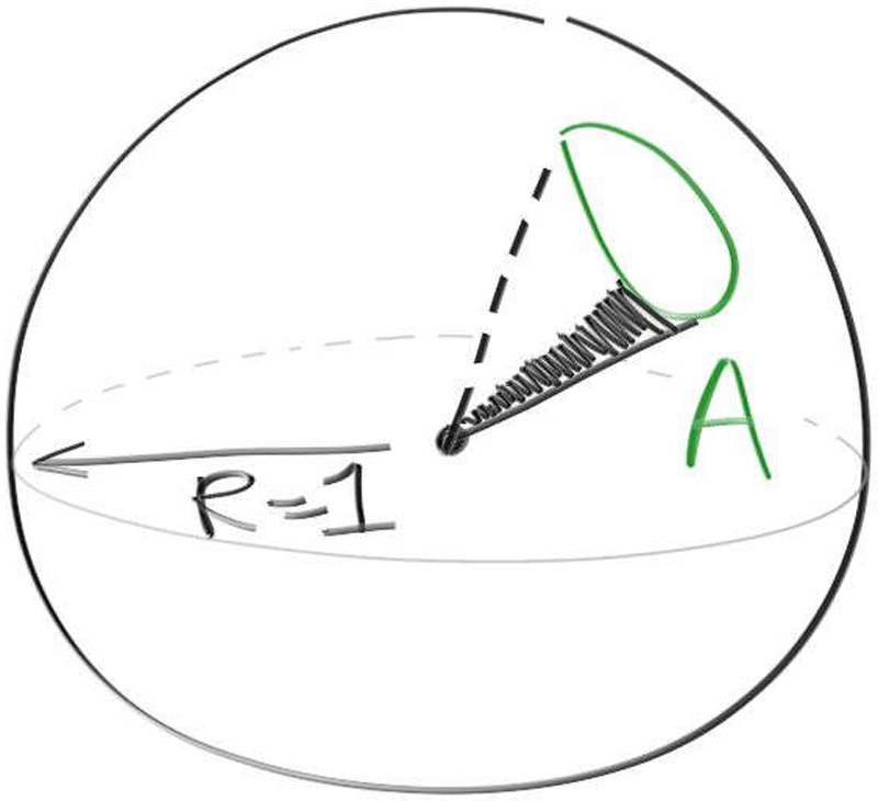
The analytic answer is $\frac{4}{3} \pi$ -- if you remember enough advanced calc, check me! And the code above produces that. The key point here is that all of the integrals and the probability and everything else is over the unit sphere. The way to represent a single direction in 3D is its associated point on the unit sphere. The way to represent a range of directions in 3D is the amount of area on the unit sphere that those directions travel through. Call it direction, area, or solid angle -- it’s all the same thing. Solid angle is the term that you'll usually find in the literature. You have radians (r) in $\theta$ over one dimension, and you have steradians (sr) in $\theta$ and $\phi$ over two dimensions (the unit sphere is a three dimensional object, but its surface is only two dimensional). Solid Angle is just the two dimensional extension of angles. If you are comfortable with a two dimensional angle, great! If not, do what I do and imagine the area on the unit sphere that a set of directions goes through. The solid angle $\omega$ and the projected area $A$ on the unit sphere are the same thing.
Now let’s go on to the light transport equation we are solving.